Worksheet 2 — Implementing Finite Element Model Classes
Introduction
In this worksheet, you will develop the core classes for a finite element analysis program. The goal is to create a modular, object-oriented structure that can be extended in future assignments. By completing this worksheet, you will have a working finite element application capable of solving basic problems in thermal conductivity, groundwater flow, or stress calculation.
The following problem types can be chosen (only one is to be implemented):
- Thermal Conductivity
- Groundwater Flow
- Stress Calculation (Plane Stress)
The selected problem will then be used for all further worksheets. You do not need to implement a program that handles all problem types.
Prerequisites:
- Basic Python knowledge including functions and classes
- Understanding of NumPy arrays and operations
Learning Objectives:
- Implement a structured object-oriented classes for implementing a finite element analysis
- Create classes for model parameters, computation, results, and reporting
- Implement file reading and writing using JSON
Structuring of a finite element code
Software development is a time-consuming job. It is therefore important that the program code is designed in such a way that modification and further development can be facilitated. This means that software programs must be structured and have good readability. A calculation process can generally be divided into different logical parts. In this application we will divide up the program into the following logical parts:
- Input data management - Handled by the ModelParams class
- Computation - Implemented in the ModelSolver class
- Results storage - Managed by the ModelResult class
- Output presentation - Provided by the ModelReport class
To improve program readability:
- Choose variable and subroutine names carefully so that they clearly describe their function.
- Use comments in each subroutine to explain the purpose, meaning, and parameters of the computational steps.
By following these guidelines, the program becomes easier to modify or repurpose for other applications.
Program architecture
Your finite element analysis program will consist of 4 main classes:
| Class | Purpose |
|---|---|
| ModelParams | Stores input parameters required for calculation |
| ModelSolver | Implements solution algorithm for the chosen problem |
| ModelResult | Stores calculation results for later use |
| ModelReport | Generates formatted reports of inputs and outputs |
We begin by defining a python-module, flowmodel.py (choose a name depending on the selected problem type), which will include the calculation part of the program. At the beginning of the file, the following declarations for the modules to be used:
# -*- coding: utf-8 -*-

import numpy as np
import calfem.core as cfc
import calfem.utils as cfu
import tabulate as tab
All classes in this worksheet will be implemented in the flowmodel.py file.
Important
When ** ... ** appears in the program examples, this indicates that there is no code that you yourselves must add. Variables and data structures are only examples. Depending on the type of problem you may need other data structures than those described in the code examples.
Important
It could be a good idea to implement the module as simple CALFEM Python script before implementing it in the classes in the sections below. This will help you to understand the problem and how to implement it in Python. You can then use the code in the module as a template for the classes.
The ModelParams-class
The ModelParams class will be used to store all input data required for the calculation as member variables. The class will have a constructor, __init__(...), which will initialize all variables to default values, ensuring that the program runs without errors.
The class input data must contain all inputs required to perform the calculation. The following code shows how the structure of the ModelParams class might look like, with all necessary variables initialized:
# -*- coding: utf-8 -*-

import numpy as np
import calfem.core as cfc
import calfem.utils as cfu
import tabulate as tab
import json

class ModelParams:
    """Class defining the model parameters"""
    def __init__(self):

        self.version = 1

        self.t = 1
        self.ep = [self.t]

        # --- Element properties

        ...

        # --- Create input for the example use cases

        self.coord = np.array([
            [0.0, 0.0],
            [0.0, 0.12],
            ...
            [0.24, 0.12]
        ])

        # --- Element topology

        self.edof = np.array([
            [...],
            ...
            [...]
        ])

        # --- Loads

        self.loads = [
            [5, 6.0],
            [6, 6.0]
        ]

        # --- Boundary conditions

        self.bcs = [
            [1, -15.0],
            [2, -15.0]
        ]
Important
All ... indicates that the code must be added.
The ModelResult-class
The ModelResult class is used to store the results generated during the calculation. Since Python is a dynamic language, it allows adding result variables to the class object during runtime. However, it is recommended to create empty variables in the class beforehand to ensure that it functions independently. An example of the ModelResult class is shown in the following code:
class ModelResult:
    """Class for storing results from calculations."""
    def __init__(self):
        self.a = None
        self.r = None
        self.ed = None
        self.qs = None
        self.qt = None
Good to know
None can be used as a generic data type that can be used to create variables without content. It is also possible to test if a variable is assigned by an if statement:
if self.a == None:
    self.a = np.array(...) # Assign a proper data type if self.a == None
The ModelSolver-class
The class ModelSolver is responsible for performing the actual calculation. The class will have a constructor, init(...) and a method execute() to perform the actual calculation. Constructor must have two input parameters, model_params and model_result, which are instances of the classes ModelParams and ModelResult. The constructor will look like the following:
class Solver:
    """Class for performing the model computations."""
    def __init__(self, model_params, model_result):
        self.model_params = model_params
        self.model_result = model_result
The input parameters are assigned two class variables, self.model_params and self.model_result.
The calculation should be performed in the execute(...) method. The method uses the input parameters from self.model_params to set up and perform finite element calculations just like a regular CALFEM. To simplify management of input variables we create local references to the input data variable as shown in the following code:
class Solver:

    ...

    def execute(self):

        # --- Assign shorter variable names from model properties

        edof = self.model_params.edof
        coord = self.model_params.coord
        dof = self.model_params.dof
        ep = self.model_params.ep
        loads = self.model_params.loads
        bcs = self.model_params.bcs
Because Python handles all variables by reference, there is no disadvantage to making these assignments. No copies of the data will be created, and the local variables will directly reference the same memory as the parameters in the self.model_params variable, eliminating the need to copy them back.
After the calculation is completed, the self.model_result is assigned the result of the calculation. The global stiffness matrix, K or the load vector f need not be stored here. Result variables to be stored are the displacement vector, the reaction force vector and the element forces. The following code shows how this might look like:
class Solver:

    ...

    def execute(self):

        # --- Assign shorter variable names from model properties

        ...

        ... Beräkningskod ...

        # --- Store results in model_results

        self.model_result.a = a
        self.model_result.r = r
        self.model_result.ed = ed
        self.model_result.qs = qs
        self.model_result.qt = qt
cfc.solveq() load and boundary conditions
cfc.solveq(...) uses a different format of loads and boundary conditions compared to what we use in the model. To convert to the correct arguments use the following example as a template:
    for load in loads:
        dof = load[0]
        mag = load[1]
        f[dof - 1] = mag

    bc_prescr = []
    bc_value = []

    for bc in bcs:
        dof = bc[0]
        value = bc[1]
        bc_prescr.append(dof)
        bc_value.append(value)

    bc_prescr = np.array(bc_prescr)
    bc_value = np.array(bc_value)

    a, r = cfc.solveq(K, f, bc_prescr, bc_value)
Extracting and storing results from elements
To utilize the results from the elements, array operations are required since the output format of the element routines may vary.
The ModelReport-class
When the calculation is completed, the ModelReport class generates a report of input parameters and results. This class uses the same input parameters as the ModelSolver class.
To generate the report, we use Python's built-in __str__() method, which defines the behavior when an instance of the class is passed to print(...) or converted to a string using str(...).
To implement this, we need two additional methods and a string variable. The string variable will store the text description of the class, while the methods will handle clearing and populating the string. The following code shows the implementation of the ModelReport class:
class ModelReport:
    """Class for presenting input and output parameters in report form."""
    def __init__(self, model_params, model_result):
        self.model_params = model_params
        self.model_result = model_result
        self.report = ""

    def clear(self):
        self.report = ""

    def add_text(self, text=""):
        self.report+=str(text)+"\n"

    def __str__(self):
        self.clear()
        self.add_text()
        self.add_text("-------------- Model input ----------------------------------")
        ...
        self.add_text("Coordinates:")
        self.add_text()
        self.add_text(
            tab.tabulate(self.params.coords, headers=["x", "y"], tablefmt="psql")
        )
        ...
        return self.report
Combining multiple arrays for tabulate
Sometimes you want to combine multiple arrays into a single table, such as displacements and reactions. This can be done using the NumPy commands np.hstack(...) and np.vstack(...). Below is an example of how to achieve this:
a_and_r = np.hstack((a, r))

temp_table = tab.tabulate(
    np.asarray(a_and_r),
    headers=["D.o.f.", "Phi [m]", "q [m^2/day]"],
    numalign="right",
    floatfmt=".4f",
    tablefmt="psql",
    showindex=range(1, len(a_and_r) + 1),
)
Main program
For the program to function correctly, we need a main program. The following code demonstrates how to implement a main program in Python:
# -*- coding: utf-8 -*-

if __name__ == "__main__":
    print("This will is executed as a script and not imported.")
If a Python file is imported with the import statement, the variable __name__ will contain the module name, i.e., the name of the source file. However, if you call the file directly with a Python interpreter, __name__** will contain the value __main__. In this way, you can ensure that only certain code is executed if the file is started directly with the Python interpreter and at the same time use the file as a module. This concept is often used in Python to create test functions for modules.
A main program of our finite element program that uses all of our classes can then look like this (ensure the class names and imports match your implementation):
# -*- coding: utf-8 -*-

import flowmodel as fm

if __name__ == "__main__":

    model_params = fm.ModelParams()
    model_result = fm.ModelResult()

    solver = fm.ModelSolver(model_params, model_result)
    solver.execute()

    report = fm.ModelReport(model_params, model_result)
    print(report)
In the above main program, we import the module flowmodel (flowmodel.py) that implements our classes. We import the module as fm. fm.ModelParams and fm.ModelResult are created to manage our input parameters and results. A ModelSolver-instance, the fm.ModelSolver is created with the parameters, model_params and model_result as input. The calculation is then started by calling the methods solver.execute(). We end the program by creating a fm.ModelReport object which we display on the screen with the print() statement.
Example of a running program is shown below:
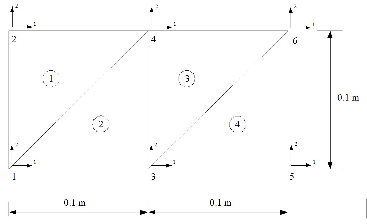
# Model report

## Input parameters

+-----+------+------+
|   t |   l1 |   l2 |
|-----+------+------|
| 0.2 |  1.7 | 0.04 |
+-----+------+------+

### Coords

+------+------+
|    x |    y |
|------+------|
| 0    | 0    |
| 0    | 0.12 |
| 0.12 | 0    |
| 0.12 | 0.12 |
| 0.24 | 0    |
| 0.24 | 0.12 |
+------+------+

### Dofs

+--------+
|   dof1 |
|--------|
|      1 |
|      2 |
|      3 |
|      4 |
|      5 |
|      6 |
+--------+

### Edof

+-------+-------+-------+
|   el1 |   el2 |   el3 |
|-------+-------+-------|
|     1 |     4 |     2 |
|     1 |     3 |     4 |
|     3 |     6 |     4 |
|     3 |     5 |     6 |
+-------+-------+-------+

### Loads

+-------+-------+
|   dof |   mag |
|-------+-------|
|     5 |     6 |
|     6 |     6 |
+-------+-------+

### BCs

+-------+---------+
|   dof |   value |
|-------+---------|
|     1 |     -15 |
|     2 |     -15 |
+-------+---------+

## Results

### Nodal temps and flows (a and r)

+----------+----------------+-----------+
|   D.o.f. |   Temp [Deg C] |   q [W/m] |
|----------+----------------+-----------|
|        1 |       -15.0000 |   -6.0000 |
|        2 |       -15.0000 |   -6.0000 |
|        3 |        20.2941 |    0.0000 |
|        4 |        20.2941 |    0.0000 |
|        5 |      1520.2941 |    0.0000 |
|        6 |      1520.2941 |    0.0000 |
+----------+----------------+-----------+

### Element flows

+-----------+-------------+-------------+
|   Element |   q_x [W/m] |   q_y [W/m] |
|-----------+-------------+-------------|
|         1 |   -500.0000 |     -0.0000 |
|         2 |   -500.0000 |      0.0000 |
|         3 |   -500.0000 |      0.0000 |
|         4 |   -500.0000 |      0.0000 |
+-----------+-------------+-------------+

### Element gradients

+-----------+------------+-----------+
|   Element |    g_x [-] |   g_y [-] |
|-----------+------------+-----------|
|         1 |   294.1176 |    0.0000 |
|         2 |   294.1176 |    0.0000 |
|         3 | 12500.0000 |   -0.0000 |
|         4 | 12500.0000 |    0.0000 |
+-----------+------------+-----------+

### Element temps

+-----------+---------------+---------------+---------------+
|   Element |   T_1 [deg C] |   T_2 [deg C] |   T_3 [deg C] |
|-----------+---------------+---------------+---------------|
|         1 |      -15.0000 |       20.2941 |      -15.0000 |
|         2 |      -15.0000 |       20.2941 |       20.2941 |
|         3 |       20.2941 |     1520.2941 |       20.2941 |
|         4 |       20.2941 |     1520.2941 |     1520.2941 |
+-----------+---------------+---------------+---------------+
# Model report

## Input parameters

+-----+-----+
|   t |   k |
|-----+-----|
|   1 |  50 |
+-----+-----+

### Coords

+------+-----+
|    x |   y |
|------+-----|
|    0 |   0 |
|    0 | 600 |
|  600 |   0 |
|  600 | 600 |
| 1200 |   0 |
| 1200 | 600 |
+------+-----+

### Dofs

+--------+
|   dof1 |
|--------|
|      1 |
|      2 |
|      3 |
|      4 |
|      5 |
|      6 |
+--------+

### Edof

+-------+-------+-------+
|   el1 |   el2 |   el3 |
|-------+-------+-------|
|     1 |     4 |     2 |
|     1 |     3 |     4 |
|     3 |     6 |     4 |
|     3 |     5 |     6 |
+-------+-------+-------+

### Loads

+-------+-------+
|   dof |   mag |
|-------+-------|
|     6 |  -400 |
+-------+-------+

### BCs

+-------+---------+
|   dof |   value |
|-------+---------|
|     2 |      60 |
|     4 |      60 |
+-------+---------+

## Results

### Nodal temps and flows (a and r)

+----------+-----------+---------------+
|   D.o.f. |   Phi [m] |   q [m^2/day] |
|----------+-----------+---------------|
|        1 |   59.0588 |        0.0000 |
|        2 |   60.0000 |       23.5294 |
|        3 |   58.1176 |        0.0000 |
|        4 |   60.0000 |      376.4706 |
|        5 |   53.4118 |       -0.0000 |
|        6 |   48.7059 |        0.0000 |
+----------+-----------+---------------+

### Element flows

+-----------+-----------------+-----------------+
|   Element |   q_x [m^2/day] |   q_y [m^2/day] |
|-----------+-----------------+-----------------|
|         1 |         -0.0000 |         -0.0784 |
|         2 |          0.0784 |         -0.1569 |
|         3 |          0.9412 |         -0.1569 |
|         4 |          0.3922 |          0.3922 |
+-----------+-----------------+-----------------+

### Element gradients

+-----------+-----------+-----------+
|   Element |   g_x [-] |   g_y [-] |
|-----------+-----------+-----------|
|         1 |    0.0000 |    0.0016 |
|         2 |   -0.0016 |    0.0031 |
|         3 |   -0.0188 |    0.0031 |
|         4 |   -0.0078 |   -0.0078 |
+-----------+-----------+-----------+

### Element temps

+-----------+-------------+-------------+-------------+
|   Element |   phi_1 [m] |   phi_2 [m] |   phi_3 [m] |
|-----------+-------------+-------------+-------------|
|         1 |     59.0588 |     60.0000 |     60.0000 |
|         2 |     59.0588 |     58.1176 |     60.0000 |
|         3 |     58.1176 |     48.7059 |     60.0000 |
|         4 |     58.1176 |     53.4118 |     48.7059 |
+-----------+-------------+-------------+-------------+
# Model report

## Input parameters

+------+----------+------+
|    t |        E |    v |
|------+----------+------|
| 0.01 | 2.08e+10 | 0.35 |
+------+----------+------+

### Coords

+-----+-----+
|   x |   y |
|-----+-----|
| 0   | 0   |
| 0   | 0.1 |
| 0.1 | 0   |
| 0.1 | 0.1 |
| 0.2 | 0   |
| 0.2 | 0.1 |
+-----+-----+

### Dofs

+--------+--------+
|   dof1 |   dof2 |
|--------+--------|
|      1 |      2 |
|      3 |      4 |
|      5 |      6 |
|      7 |      8 |
|      9 |     10 |
|     11 |     12 |
+--------+--------+

### Edof

+-------+-------+-------+-------+-------+-------+
|   el1 |   el2 |   el3 |   el4 |   el5 |   el6 |
|-------+-------+-------+-------+-------+-------|
|     1 |     2 |     7 |     8 |     3 |     4 |
|     1 |     2 |     5 |     6 |     7 |     8 |
|     5 |     6 |    11 |    12 |     7 |     8 |
|     5 |     6 |     9 |    10 |    11 |    12 |
+-------+-------+-------+-------+-------+-------+

### Loads

+-------+--------+
|   dof |    mag |
|-------+--------|
|    12 | -10000 |
+-------+--------+

### BCs

+-------+---------+
|   dof |   value |
|-------+---------|
|     1 |       0 |
|     2 |       0 |
|     3 |       0 |
|     4 |       0 |
+-------+---------+

## Model results


### Displacements and reactions

+-------+----------------------+-----------------------+
|   DOF |   Displacements [mm] |   Reaction force [kN] |
|-------+----------------------+-----------------------|
|     1 |               0.0000 |               20.0000 |
|     2 |               0.0000 |               -2.5031 |
|     3 |               0.0000 |              -20.0000 |
|     4 |               0.0000 |               12.5031 |
|     5 |              -0.1052 |                0.0000 |
|     6 |              -0.2423 |                0.0000 |
|     7 |               0.0973 |               -0.0000 |
|     8 |              -0.2198 |                0.0000 |
|     9 |              -0.1262 |               -0.0000 |
|    10 |              -0.5736 |                0.0000 |
|    11 |               0.1178 |                0.0000 |
|    12 |              -0.5946 |                0.0000 |
+-------+----------------------+-----------------------+

### Element displacements

+-------+------------+------------+------------+------------+------------+------------+
|   el. |   ed1 [mm] |   ed2 [mm] |   ed3 [mm] |   ed4 [mm] |   ed5 [mm] |   ed6 [mm] |
|-------+------------+------------+------------+------------+------------+------------|
|     1 |     0.0000 |     0.0000 |     0.0973 |    -0.2198 |     0.0000 |     0.0000 |
|     2 |     0.0000 |     0.0000 |    -0.1052 |    -0.2423 |     0.0973 |    -0.2198 |
|     3 |    -0.1052 |    -0.2423 |     0.1178 |    -0.5946 |     0.0973 |    -0.2198 |
|     4 |    -0.1052 |    -0.2423 |    -0.1262 |    -0.5736 |     0.1178 |    -0.5946 |
+-------+------------+------------+------------+------------+------------+------------+

### Element stresses

+-------+-------------+-------------+-------------+
|   el. |   es1 (MPa) |   es2 (MPa) |   es3 (Mpa) |
|-------+-------------+-------------+-------------|
|     1 |     23.0674 |      8.0736 |    -16.9326 |
|     2 |    -23.0674 |     -3.3852 |     -3.0674 |
|     3 |      6.7242 |      7.0419 |    -13.2758 |
|     4 |     -6.7242 |     -6.7242 |     -6.7242 |
+-------+-------------+-------------+-------------+

### Element strains:

+-------+------------+------------+------------+
|   el. |   et1 [mm] |   et2 [mm] |   et3 [mm] |
|-------+------------+------------+------------|
|     1 |     0.9732 |     0.0000 |    -2.1980 |
|     2 |    -1.0520 |     0.2254 |    -0.3982 |
|     3 |     0.2048 |     0.2254 |    -1.7233 |
|     4 |    -0.2101 |    -0.2101 |    -0.8729 |
+-------+------------+------------+------------+
Reading and writing to a file using JSON
An important part of a calculation program is being able to read and write input files. In most cases, the problems are so large that they can not be defined in the program code. In this program, we will use JSON (JavaScript Object Notation) as the format of the files we will write. The following code is an example of how a JSON file might look like:
{"employees":[
    {"firstName":"John", "lastName":"Doe"},
    {"firstName":"Anna", "lastName":"Smith"},
    {"firstName":"Peter", "lastName":"Jones"}
]}
The file format is very similar to the syntax used by Python dictionaries. This similarity makes it attractive, as Python provides a built-in library to easily read and write files in this format.
To implement the functionality for reading and writing JSON files in our program, we add the following imports at the beginning of our module file:
We start by implementing writing to a file as we have all input parameters required for this. Below is the skeleton implementation of the save() method in the ModelParams-class:
class ModelParams:
    """Class defining the model parameters."""

    ...

    def save(self, filename):
        """Save input to file."""

        ...
To define the structure of what is to be stored, but also to make it easy to read data, we will start from a dictionary as the base for what should be written and read to file. In the save()-method we add the following code to define a parameter dictionary:
        model_params = {}
        model_params["version"] = self.version
        model_params["t"] = self.t
        model_params["ep"] = self.ep
The model_params["version"] entry is a good way of keeping track of the version of the file format that is written. This can later be used to read a different version of the file correctly.
One problem we need to handle is that the JSON module can't handle NumPy arrays. This is solved by converting our numpy arrays to lists. In the following code, we convert the array self.coord to a list using the .tolist() method in NumPy.
When the input parameters have been defined, we can open a file for writing the dictionary to file using the json.dumps(...) function.
        ofile = open(filename, "w")
        json.dump(model_params, ofile, sort_keys = True, indent = 4)
        ofile.close()
sort_keys and indent ensure that the file written is nicely formatted.
To load an existing JSON file we do the procedure in reverse. We read the entire file into a string of characters which we then convert back to a dictionary function using the json.load(...)-function.
    def load(self, filename):
        """Read input from file."""

        ifile = open(filename, "r")
        model_params = json.load(ifile)
        ifile.close()

        self.version = model_params["version"]
        self.t = model_params["t"]
        self.ep = model_params["ep"]
The self.coord-array must now be converted back to a numpy array. This is done with the numpy function np.asarray(...).
The complete ModelParams class with read and write functionality is shown below:
class ModelParams:
    """Class defining the model parameters."""

    def save(self, filename):
        """Save input data to file."""

        model_params = {}
        model_params["version"] = self.version
        model_params["t"] = self.t
        model_params["ep"] = self.ep
        ...
        model_params["coord"] = self.coord.tolist()
        ...

        ofile = open(filename, "w")
        json.dump(model_params, ofile, sort_keys = True, indent = 4)
        ofile.close()

    def load(self, filename):
        """Read input data from file."""

        ifile = open(filename, "r")
        model_params = json.load(ifile)
        ifile.close()

        self.version = model_params["version"]
        self.t = model_params["t"]
        self.ep = model_params["ep"]
        ...
        self.coord = np.asarray(model_params["coord"])
        ...
Submission and accounting
To complete the worksheet you must:
- Complete the implementation of the ModelParams-class with all the required input to solve the chosen problem. Procedures to save and read from JSON files will also be implemented for all input variables.
- Complete the implementation of the ModelSolver-class with a finite element solver implemented with the methods that are described in CALFEM.
- Complete the implementation of the ModelReport-class with a complete transcript of the input and output variables with descriptive texts.
The submission shall consist of a zip file (or other archive format) consisting of:
- All the Python files. (.py Files)
- An example of a saved file JSON.
- Printing from applications run.
Element types
Plate element
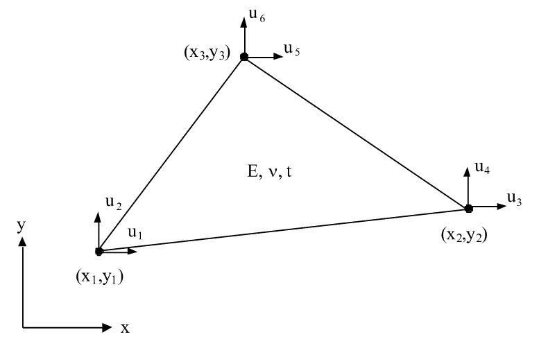
- u = displacement
- x1,y1,x2,y2,x3,y3 = coordinates
- E = Young's modulus
- v = Poisson's ratio
- CALFEM for Python element: plante/plants
2-dimensional heat flow
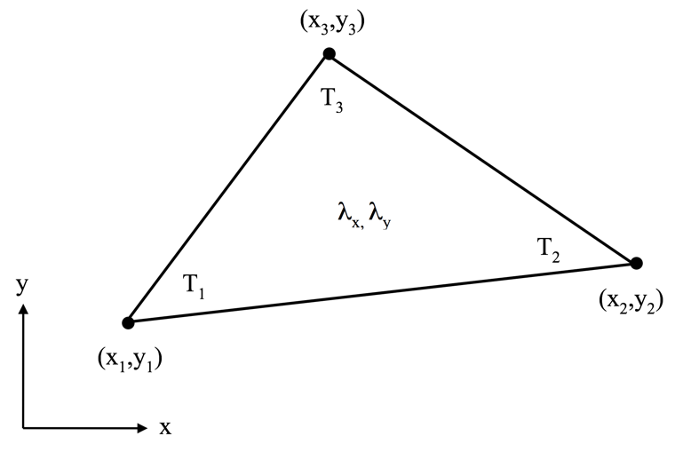
- T = temperature
- x1,y1,x2,y2,x3,y3 = coordinates
- lambda_x, lambda_y = thermal conductivity
- CALFEM for Python element: flw2te/flw2ts
Groundwater flow
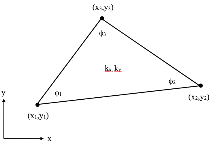
- phi = pressure head
- x1,y1,x2,y2,x3,y3 = coordinates
- kx, ky = permeabilities
- CALFEM for Python element: flw2te/flw2ts
Test examples
Plane stress
- E = 20.8 GPa
- t = 0.01 m
- R_6,2 = -10.0 kN
- u_1,1 = u_1,2 = u_2,1 = u_2,2 = 0.0
- Plane stress
- u_i,j where i is the node number and j is the local degree of freedom
Two-dimensional heat flow
- lambda_x1 = lambda_y1 = 1.7 W/mC
- lambda_x2 = lambda_y2 = 0.04 W/mC
- q_5 = q_6 = 6.0 W/m
- T_1 = T_2 = -15.0 0C
- t = 0.2 m
Groundwater flow
- k_x = k_y = 50 m/dag
- q_6 = -400 m^2/dag
- phi_2 = phi_4 = 60.0 m
- t = 1.0 m